Introducing the stationary heat equation
The stationary heat equation is a partial differential equation that describes the variation in temperature in a material in stationary conditions. In two dimension, it looks like : $$\frac{\partial ^2 T}{\partial x^2} + \frac{\partial ^2 T}{\partial y^2} = \frac{1}{k} q(x,y)$$
where :
\(k\) is the thermal conductivity (\(W.m^{-1}.K^{-1}\)) of the material studied ;
\(q\) is the heat flux density (\(W.m^{-2}\)) of the sources.
Abstract
During S6 at ENSEIRB-MATMECA, I completed 6 two-week numerical analysis projects, using Python, in teams of 5 or 6 students. The numerical solution of the stationary heat equation was one of the most interesting in my opinion, so I decided to display it here, to showcase my abilities in Python and numerical analysis.
At the time, my team did a quite good job considering the small amount of time we had. But I was not completely satisfied, so during summer 2015, I made a critical examination of our code, immerse myself into the mathematics behind it, and rewrote most of it. I also developped a simple GUI. This page presents this process and the final result, which is downloadable from this github repository.
The finite difference method
A possible approch to numerical solutions of partial differential equation is the finite-difference methods.
Basically, it is a discretization method where finite differences are used to approximate the derivatives.
Assuming the temperature function is properly-behaved, we can write thanks to Taylor theorem :
$$T(x+h,y) = T(x,y) + h \frac{\partial T}{\partial x}(x,y) + \frac{h^2}{2} \frac{\partial^2 T}{\partial x^2}(x,y) + \frac{h^3}{6} \frac{\partial^3 T}{\partial x^3}(x,y) + \frac{h^4}{24} \frac{\partial^4 T}{\partial x^4}(\eta,y)$$
$$T(x-h,y) = T(x,y) - h \frac{\partial T}{\partial x}(x,y) + \frac{h^2}{2} \frac{\partial^2 T}{\partial x^2}(x,y) - \frac{h^3}{6} \frac{\partial^3 T}{\partial x^3}(x,y) + \frac{h^4}{24} \frac{\partial^4 T}{\partial x^4}(\zeta,y)$$
where \(\eta \in [x, x+h]\) and \(\zeta \in [x-h, x]\), then by adding both equations :
$$\frac{\partial ^2 T}{\partial x^2}(x,y) = \frac{T(x+h, y) - 2T(x,y) + T(x-h, y)}{h^2} + \frac{h^2}{24} \Big (\frac{\partial^4 T}{\partial x^4}(\eta,y) + \frac{\partial^4 T}{\partial x^4}(\zeta,y)\Big)$$
Finally, by doing the same thing on the other axis, and disregarding the fourth and upper order terms when \(h\) is small enough, we can rewrite the stationnary heat equation as :
$$ \frac{T(x+h, y) + T(x, y+h) - 4T(x,y) + T(x-h, y) + T(x-h, y)}{h^2} = \frac{1}{k} q(x,y) $$
Now let us assume we want to solve the 2-D stationnary heat equation on a surface \( [a,b] \times [a,b] \).
To solve it numerically, we discretize the space in a \(n\times n \) matrix of regularly spaced points.
As a consequence, the heat flux density field is also discretized, and represented by a \(n\times n \) matrix Q, such as \(\forall (i,j), \ q_{i,j} = q(i*h,j*h)\).
Finally, an approximation of the temperature field in all the discrete points, in the form of a \(n\times n \) matrix T, such as \(\forall (i,j), \ t_{i,j} \simeq T(i*h,j*h)\), is obtained by considering the set of \((n-2)*(n-2)\) equations :
$$ \forall (i,j) \in [[1,n-2]]\times[[1,m-2]], \ \frac{t_{i+1,j} + t_{i,j+1} + 4_{i,j} + t_{i-1,j} + t_{i,j-1}}{h^2} = \frac{1}{k} q_{i,j} $$
and the \(4(n-1)\) boundary conditions.
Let us note \(matToVect()\) the operator transforming a \(n\times n\) matrix into a \(n*n\) column vector whose \(i\)-th coefficient is the \((i/n, i\%n)\) coefficient of the matrix, and \(vectToMat()\) the reverse operator.
By choosing null boundary conditions, this system of \(n^2\) linear equations can be put in the form of a matrix system : \(Ax= matToVect(Q)\) where
$$A=\begin{bmatrix} B & C \\ C & B &\ddots \\ &\ddots & \ddots & C \\ & & C & B \end{bmatrix}
\
\text{with }
B= \begin{bmatrix} -4 & 1 \\ 1 & -4 &\ddots \\ &\ddots & \ddots & 1 \\ & & 1 & -4 \end{bmatrix}
\text{ , }
C= I_n
\text{ , } T = vectToMat(x) $$
Cholesky factorization
The matrix \(A\) described above has an interesting characteristic : \(-A\) is symmetric and positive definite. Now, if a matrix \(M\) is symmetric positive definite, it has a decomposition called Cholesky factorization of the form \(M = LL^*\) where \(L\) is a lower triangular matrix and \(L^*\) is its transpose. This decomposition, which can be performed in \(\Theta(n^3)\) for a \(n\times n\) matrix, is very useful, as it allows to solve very efficiently and with great numerical stability \(Ax = col(Q)\) by solving two triangular linear systems (\(Ly=col(Q)\) then \(-L^*x=y\)).
There are several algorithm that perform this factorization, but one of the fastest is the Cholesky–Crout algorithm, which computes coefficients of \(L\) one by one, starting from the upper left corner, and proceeding column by column, thanks to the following formulas :
$$ L_{j,j} = \sqrt{A_{j,j} - \sum_{k=0}^{j-1} L^2_{j,k}}$$
$$ L_{i,j} = \frac{1}{L_{j,j}} \Big (A_{i,j} - \sum_{k=0}^{j-1} L_{i,k} L_{j,k} \Big) \ \text{for } i > j$$
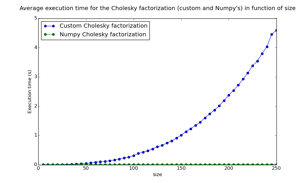
The first implementation of this algorithm made by my team was pretty slow, and as a result, we could only use it on small matrices, resulting in poor approximations. I first tried to optimize it by concatenating some loops, and removing intermediate variables and functions. The resulting function, that you can found under the name oldCompleteCholesky, was slightly faster, but still very slow for a \(\Theta(n^3)\) ...
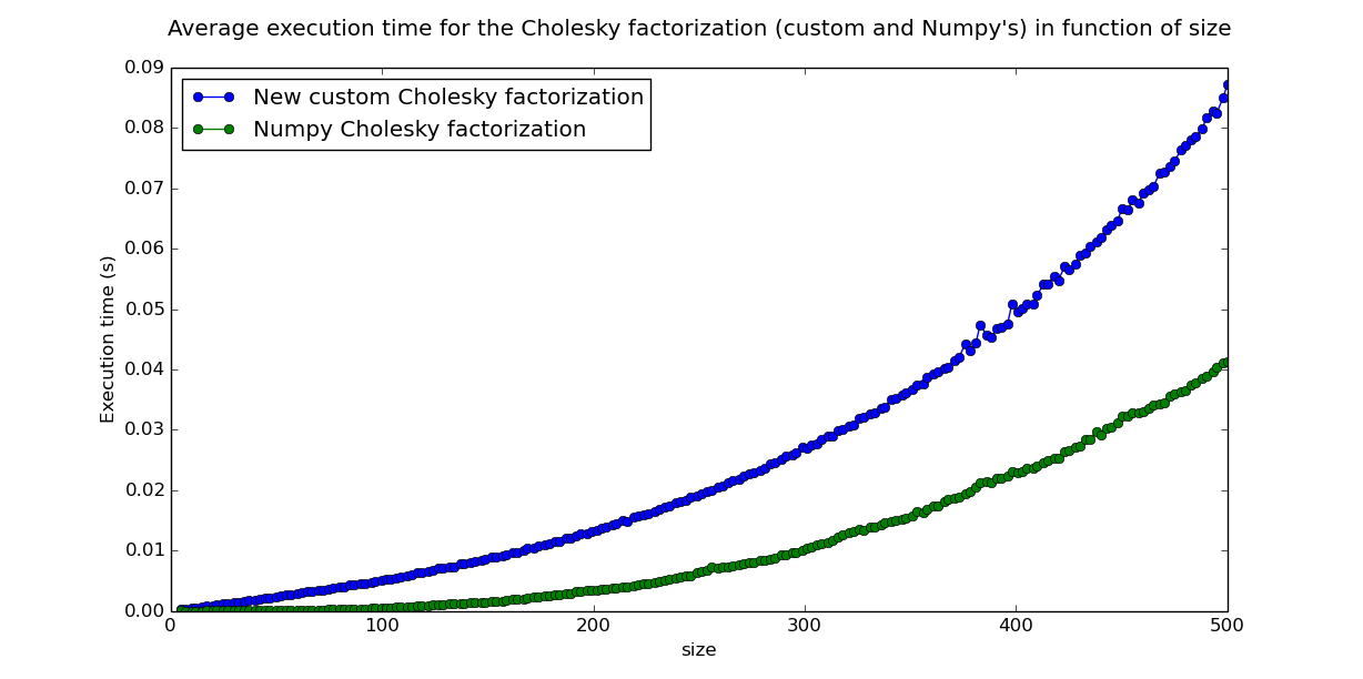
After some research, I became aware of this existence of a Cholesky factorization function in Numpy, a library I had been using for matrix computations. I compared its execution time with my custom function and the result puzzled me : my function was so slow, that Numpy's seemed to be running in constant time in comparison.
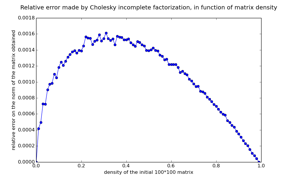
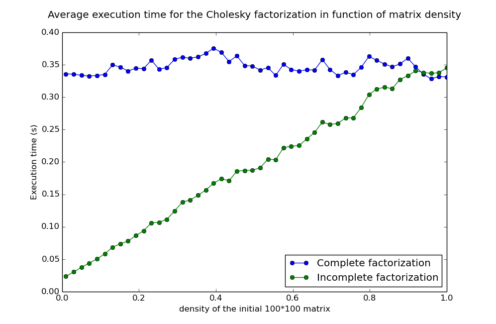
I explored another lead, which was using the incomplete Cholesky factorization, which gives a good approximation for sparse matrices like A (which density is only a few percents, and decreases with its size). As you can see, it was faster, and gave a very close approximation, but it still was not as fast as Numpy's function, which gave exact results !
I read Numpy's function source code and found out the origin of my problem. Numpy's Python Cholesky function is just a kind of wrapper for a C function, which itself make calls to the LAPACK, a Fortran library developped by american academics.
I then understood that I was not using Python in the "right" way, performance wise. Python is developped in C, and performing Python loops over the matrices coefficient is far slower than using standard functions which perform C loops and give the same result !
So, in completeCholeskyI replaced every loop I could by matrix multiplications, and reached half the speed of Numpy's function !
Solution
I developped the final solving function using Numpy's functions which were (of course) still faster. The file heatEquation.py contains the function heatEquationMatrix which produces the matrix A described above, the functions matToVect and vectToMat. The function solveHeatEquation uses them, as well as Numpy's cholesky and solve_triangular, to solve the stationary heat equation.
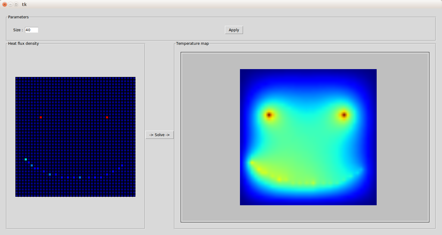
Finally, I used Python standard GUI package, Tkinter, to wrap the solving function in a simple interface. It is very simple to use : choose the size of the discretized plane you want to work on, then draw the heat flux density by clicking on the grid and click on the solve button.